
Belief Distribution Learning — an extension to Evidential Deep Learning
What do these have in common?
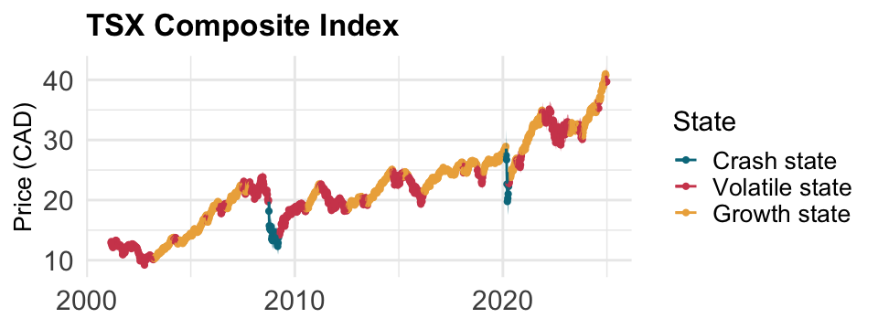
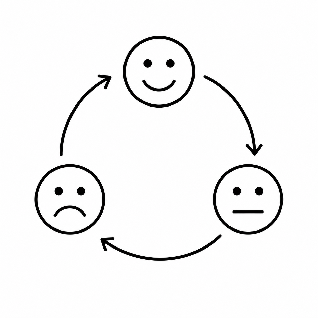
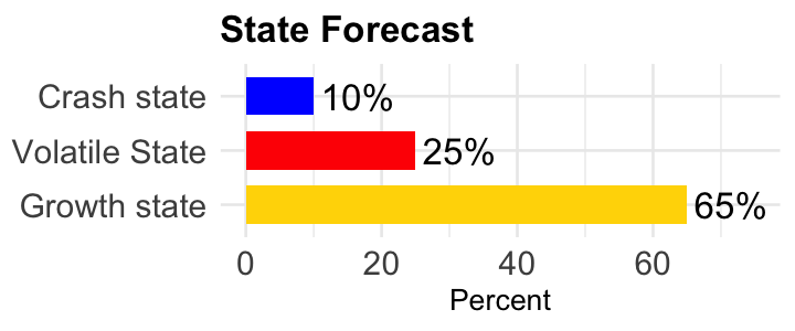
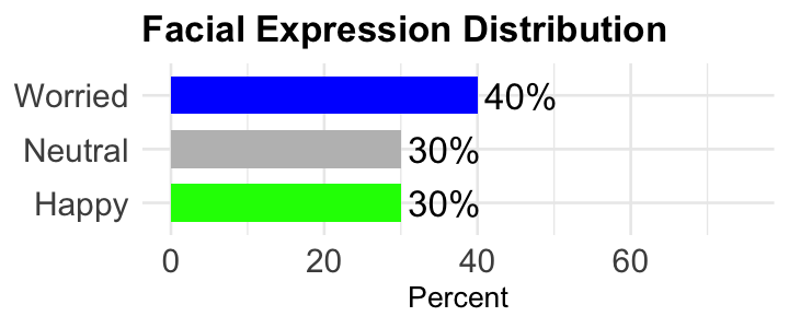
Research Goal
Develop an uncertainty aware Deep Learning classifier for LDL applications.
- Prioritize accuracy
- Provide calibrated uncertainty estimation
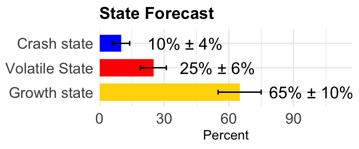
vs
Evidential Deep Learning
Generic Prediction
Softmax prediction output:
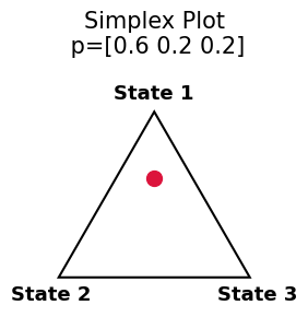
Evidential Deep Learning
Dirichlet distribution output:
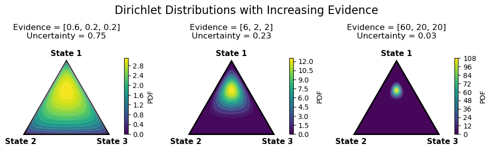
Evidential Deep Learning
In Evidential Deep Learning [Sensoy 2018], a neural network with a ReLU output layer learns an evidence vector \(\mathbf{e}\) that parametrizes a Dirichlet Distribution.
Step 1: The network maps inputs to evidence:
\[ \mathbf{e} = f_{\hat\theta}(X) \qquad (\text{ReLU ensures } e_i \geq 0) \]Step 2: Evidence defines the Dirichlet parameters:
\[ \begin{aligned} \alpha_i &= e_i + 1 \quad \forall i \in K \\ \text{Dir}(\mathbf{p}, \boldsymbol{\alpha}) &= \frac{1}{B(\alpha)}\prod_{i=1}^{K} p_i^{\alpha_i-1} \\ \text{Model Uncertainty}: u &= \frac{K}{\sum_{i=1}^K \alpha_i} \end{aligned} \]Evidential Deep Learning
The Problem: Learned evidence vectors treat each class independently and ignore the simplex constraint.
Because probabilities must sum to one, evidence towards one class requires reduced evidence towards the other classes.
Example: If the model is certain that \(p_1 = 1\), then it must be equally certain that \(p_2 = 0\), but standard EDL does not enforce this.
Belief Distribution Learning
Belief Distribution Learning is derived from Subjective Logic [Jøsang 2016], which decomposes a probability into belief and uncertainty:
\[ \begin{aligned} \mathbf{P} &= \mathbf{b} + u\,\mathbf{a} \\ 1 &= u + \sum \mathbf{b} \end{aligned} \]where
- \(\mathbf{b}\) — the belief mass assigned to each outcome
- \(u\) — the uncertainty mass
- \(\mathbf{a}\) — the base rate (prior probability)
The probability of an event is your belief, plus your uncertainty distributed according to the prior.
Belief Distribution Learning
We propose Belief Distribution Learning, where a deep learning model predicts the belief \(\mathbf{b}\) and uncertainty \(u\) through a softmax output layer.
\[ u, \mathbf{b} = f_{\hat\theta}(X) \qquad \left(\text{Softmax ensures } \textstyle\sum b_i + u = 1\right) \]These outputs map to Dirichlet parameters, which provide uncertainty quantification:
\[ \alpha_i = \frac{1}{K}\left( \frac{b_i}{u} + \bar{p}_i \right) + 1 \]where \(K\) is the number of classes, and \(\bar{p}_i\) is the average class probability over the training data.
Belief Distribution Learning
Example PDF plots
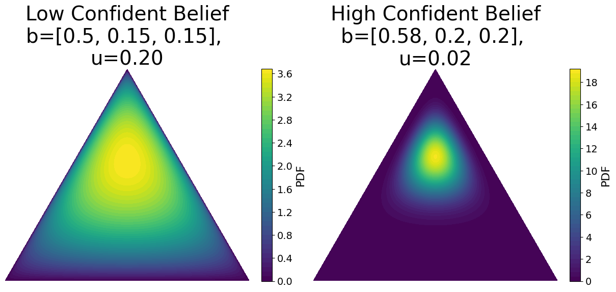
BDL Results
| Model | KL Div. \(\downarrow\) | Chebyshev \(\downarrow\) | Clark \(\downarrow\) | Canberra \(\downarrow\) |
|---|---|---|---|---|
| BDL | 0.042±0.003 | 0.087±0.004 | 0.319±0.009 | 0.654±0.019 |
| EDL | 0.053±0.004 | 0.103±0.004 | 0.357±0.010 | 0.741±0.023 |
| DP | 0.073±0.004 | 0.119±0.005 | 0.424±0.012 | 0.886±0.026 |
| SNEFY | 0.136±0.011 | 0.146±0.007 | 0.566±0.021 | 1.172±0.044 |
BDL (ours): Belief Distribution Learning · EDL: Evidential Deep Learning [Sensoy 2018] · DP: Direct Prediction · SNEFY: Squared Neural Family [Zhang 2025]
multi-Belief Distribution Learning
The Idea: What if we deconstruct multi label learning into K single label learners.
- Each learner is a 1 vs rest classifier
- The learners are constrained to the simplex using belief logic
From belief logic we define:
\[ \begin{aligned} p_i &= b_i + u_i \quad \forall i \in K \\ 1 &= \sum_{i=1}^K b_i + u_i \\ \mathbf{b}, \mathbf{u} &= f_{\hat\theta}(X) \quad \left(\text{Softmax}\right) \end{aligned} \]Multi-Belief Distribution Learning
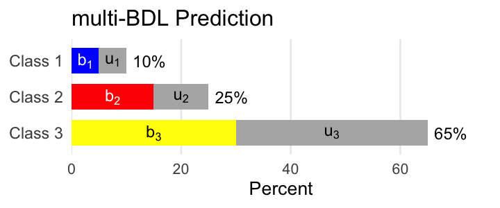
Construct \(K\) Beta distributions (one-vs-rest):
- Class \(i\): \(\;\alpha_i = \frac{1}{K}\!\left(\frac{b_i + u_i}{u_i}\right) + 1\)
- The rest: \(\;\beta_i = \frac{1}{K}\!\left(\frac{1 - b_i - u_i}{u_i}\right) + 1\)
The joint PDF is the product over labels:
\[ \text{mBDL}(\mathbf{p} \mid \boldsymbol{\alpha}, \boldsymbol{\beta}) = \prod_{i=1}^K \text{Beta}(p_i \mid \alpha_i, \beta_i) \]Multi-Label Belief Distribution Learning
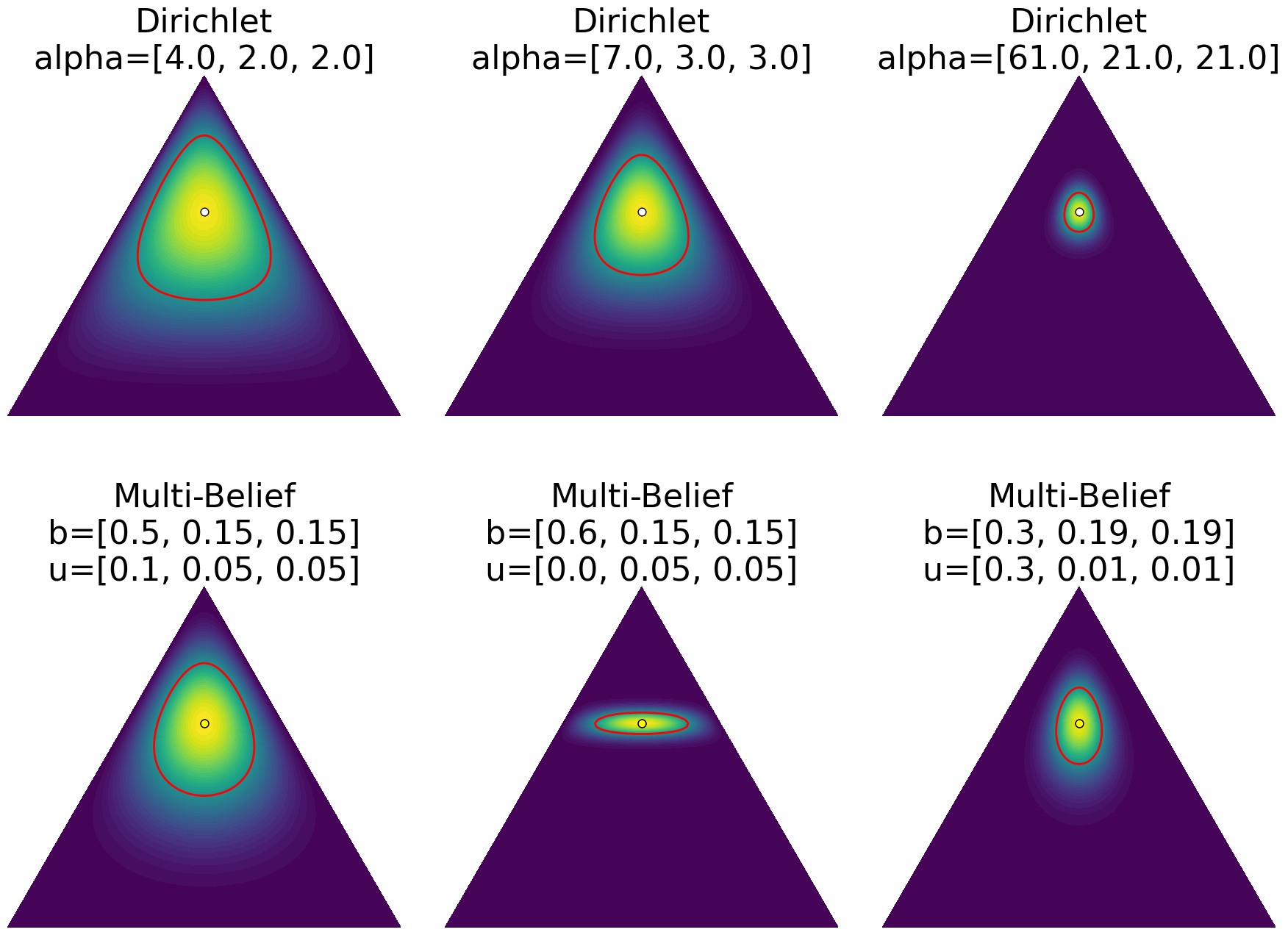
Multi-BDL has flexible confidence bounds while BDL does not.
Results
| Model | KL Div. \(\downarrow\) | Joint FSC \(\uparrow\) | Worst-Bin FSC \(\uparrow\) |
|---|---|---|---|
| BDL | 0.042±0.003 | 0.551±0.034 | 0.518±0.039 |
| multiBDL | 0.042±0.002 | 0.586±0.036 | 0.568±0.030 |
| EDL | 0.060±0.005 | 0.510±0.034 | 0.488±0.022 |
| DP | 0.073±0.004 | 0.498±0.045 | 0.547±0.031 |
| SNEFY | 0.141±0.013 | 0.571±0.045 | 0.540±0.026 |
KL Divergence: Measure of agreement between predicted and true label distribution. FSC (Feature-Stratified Coverage): Uncertainty calibration metric. Joint: combined calibration across labels; Worst-Bin: worst performing quartiles across labels.
Conclusions
- Belief theory from Subjective Logic applied to the concepts of Evidential Deep Learning improves accuracy on LDL tasks.
- Multi-belief, which allows for label specific uncertainty, improves conformal predictions compared to competing methods.
| Model | KL Div. \(\downarrow\) | Joint FSC \(\uparrow\) | Worst-Bin FSC \(\uparrow\) |
|---|---|---|---|
| BDL | 0.042±0.003 | 0.551±0.034 | 0.518±0.039 |
| multiBDL | 0.042±0.002 | 0.586±0.036 | 0.568±0.030 |
| SNEFY | 0.141±0.013 | 0.571±0.045 | 0.540±0.026 |
References
- M. Sensoy, L. Kaplan, and M. Kandemir, “Evidential Deep Learning to Quantify Classification Uncertainty,” in Advances in Neural Information Processing Systems, vol. 31, Curran Associates, Inc., 2018.
- D. Zhang, R. Tsuchida, and D. Sejdinovic, “Label Distribution Learning using the Squared Neural Family on the Probability Simplex,” in Proceedings of the Forty-first Conference on Uncertainty in Artificial Intelligence, PMLR, 2025, pp. 4872–4888.
- A. Jøsang, Subjective Logic. Artificial Intelligence: Foundations, Theory, and Algorithms, Cham: Springer International Publishing, 2016.
Results on more datasets
| Model | Dataset | KL divergence | Joint FSC | Worst-bin FSC |
|---|---|---|---|---|
| EDL | SBU_3DFE | 0.067±0.001 | 0.488±0.012 | 0.762±0.013 |
| multiBDL | SBU_3DFE | 0.067±0.001 | 0.482±0.013 | 0.790±0.010 |
| BDL | SBU_3DFE | 0.070±0.001 | 0.482±0.011 | 0.745±0.013 |
| DP | SBU_3DFE | 0.076±0.001 | 0.480±0.008 | 0.765±0.007 |
| SNEFY | SBU_3DFE | 0.409±0.050 | 0.575±0.010 | 0.734±0.018 |
Uncertainty types
Epistemic Uncertainty: When the model has insufficient information to make a confident prediction.
- •Generally dominates in out-of-distribution examples.
- ◦Example: Covid-19 was a novel environment with high epistemic uncertainty.
- →Predictions should have low confidence.
Aleatoric Uncertainty: Randomness inherent to the data itself.
- •Should lead to more probability mass spread across the hidden states.
- ◦Example: Random week-to-week swings of an asset price.
- →Predictions can have high confidence.