
Belief Distribution Learning

Research Objective
Model label distributions with accurate predictions and well-calibrated uncertainty.
Background
Label Distribution Learning (LDL) predicts a probability distribution over labels for each sample — e.g. predicting that a dog is 75% Golden Retriever and 25% Poodle.
Dirichlet Distribution is a probability distribution on the K-dimensional simplex with parameters \(\boldsymbol{\alpha}\) representing evidence toward each label:
\[ \text{Dir}(\mathbf{p} \mid \boldsymbol{\alpha}) = \frac{1}{B(\boldsymbol{\alpha})}\prod_{i=1}^K p_i^{\alpha_i - 1} \]where \(B(\boldsymbol{\alpha})\) is the multinomial Beta function. Dirichlet can be used in LDL to obtain point estimates with uncertainty.
Beta distribution is a special case of Dirichlet when \(K = 2\).
Evidential Deep Learning
In EDL [1], a neural network predicts positive evidence vectors for each label using a ReLU output which directly parameterize a Dirichlet distribution
\[ \boldsymbol{\alpha} = f_{\theta}(X)+\boldsymbol{1} \quad (\text{ReLU}) \]where \(f_{\theta}(X)\) are the neural network predictions for input \(X\) and learned parameters \(\hat\theta\).
The Problem: Each parameter is independent, violating LDL principles.
Belief Distribution Learning (ours)
In BDL, a probability estimate \(\mathbf{p}\) is decomposed into three components: belief mass \(\mathbf{b}\), uncertainty mass \(u\), and prior probability \(\boldsymbol{a}\) [2]:
\[ \begin{aligned} \mathbf{p} &= \mathbf{b} + u\boldsymbol{a} \\ 1 &= u + \sum \mathbf{b}. \end{aligned} \]A neural network with learned parameters \(\hat\theta\) predicts the belief vector and uncertainty scalar using a Softmax output,
\[ u, \mathbf{b} = f_\theta(X) \quad (\text{Softmax}), \]which parametrize a Dirichlet distribution using
\[ \boldsymbol{\alpha} = \frac{1}{K}\left(\frac{\mathbf{b}}{u} + \mathbf{a}\right) + 1. \]multi-Belief Distribution Learning (ours)
In mBDL, uncertainty is instead predicted per label
\[ \mathbf{u}, \mathbf{b} = f_\theta(X) \quad (\text{Softmax}). \]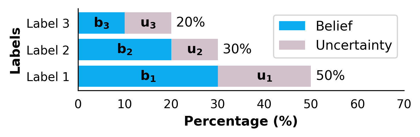
The probability estimate is
\[ \mathbf{p}=\mathbf{b}+\mathbf{u}. \]Uncertainty per label is a one-vs-rest Beta distribution:
\[ \begin{aligned} \text{one:} \quad \alpha_i &= \frac{1}{K}\!\left(\frac{b_i + u_i}{u_i}\right) + 1\\ \text{rest:} \quad \beta_i &= \frac{1}{K}\!\left(\frac{1 - (b_i + u_i)}{u_i}\right) + 1 \end{aligned} \]The joint PDF is the product over all labels:
\[ \text{mBDL}(\mathbf{p} \mid \boldsymbol{\alpha}, \boldsymbol{\beta}) = \prod_{i=1}^K \text{Beta}(p_i \mid \alpha_i, \beta_i) \]Benefit of Belief Logic
Belief logic enforces the simplex constraint. Unlike with evidence vectors, increasing belief in one label requires reducing belief in others, which directly aligns with LDL.
Results
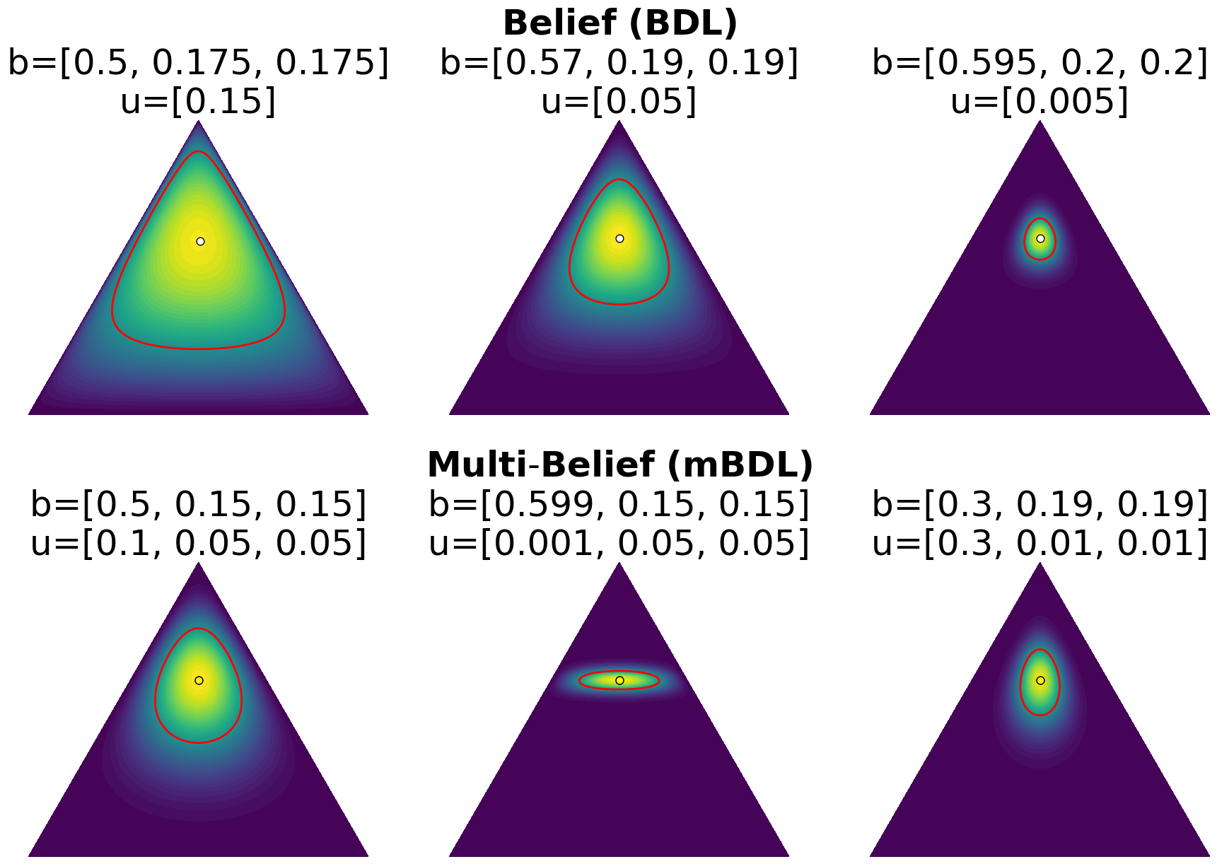
EDL (not shown) and BDL both produce symmetric Dirichlet distributions which restrict their flexibility. mBDL allows for asymmetry, providing better calibrated uncertainty.
| Model | KL Div. \(\downarrow\) | Joint FSC \(\uparrow\) | Worst-Bin FSC \(\uparrow\) |
|---|---|---|---|
| BDL | 0.042±0.003 | 0.55±0.03 | 0.52±0.04 |
| mBDL | 0.042±0.002 | 0.59±0.04 | 0.57±0.03 |
| EDL | 0.060±0.005 | 0.51±0.03 | 0.49±0.02 |
| DP | 0.073±0.004 | 0.50±0.04 | 0.55±0.03 |
| SNEFY | 0.141±0.013 | 0.57±0.04 | 0.54±0.03 |
BDL (ours): Belief Distribution Learning · mBDL (ours): multi-Belief Distribution Learning · EDL: Evidential Deep Learning · DP: Direct Prediction with Bayesian dropout for uncertainty estimates · SNEFY: Squared Neural Family [3]
Conclusion
Belief logic improves LDL accuracy and asymmetric distributions improve uncertainty calibration.
Metrics
Kullback-Leibler Divergence (KL Div.): measure of agreement between two probability vectors.
Feature Stratified Coverage (FSC): Per-label coverage of the 90% conformal region, based on calibrated conformal intervals.
Joint FSC: The 90% conformal coverage considering all labels simultaneously.
Worst-Bin FSC: Each label is split into 4 quartiles, the lowest FSC score across bins and labels is recorded.
References
- M. Sensoy, L. Kaplan, and M. Kandemir, “Evidential deep learning to quantify classification uncertainty,” in Advances in Neural Information Processing Systems, vol. 31, Curran Associates, Inc., 2018.
- A. Jøsang, Subjective Logic. Artificial Intelligence: Foundations, Theory, and Algorithms, Cham: Springer International Publishing, 2016.
- D. Zhang, R. Tsuchida, and D. Sejdinovic, “Label distribution learning using the squared neural family on the probability simplex,” in Proceedings of the Forty-first Conference on Uncertainty in Artificial Intelligence, PMLR, 2025, pp. 4872–4888.
Contact Information
- Email: dcameronsteinke@gmail.com